
Early one Sunday morning, while I was waiting for the dog path to dry off from the evening rain so that I could walk my mutts, I figured I’d take a look at multi-class classification using the LightGBM (light gradient bosting machine) system. LightGBM is a sophisticated tree-based system that can perform classification, regression, and ranking.
There are several interfaces to LightGBM. I like the easy-to-use Python scikit-learn API. LightGBM isn’t installed by default with the Anaconda Python distribution I use, so I installed it with the command “pip install lightgbm”.
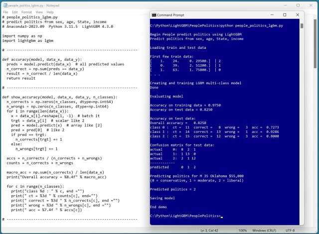
For my demo, I used one of my standard synthetic datasets. The goal is to predict political leaning from sex, age, State, and income. The 240-item tab-delimited raw data looks like:
F   24   michigan   29500.00   liberal
M   39   oklahoma   51200.00   moderate
F   63   nebraska   75800.00   conservative
M   36   michigan   44500.00   moderate
F   27   nebraska   28600.00   liberal
. . .
For LightGBM, it’s best to use ordinal encoding for categorical predictor variables. I encoded the sex variable as M = 0 and F = 1. I encoded State as Michigan = 0, Nebraska = 1, Oklahoma = 2. I encoded politics as conservative = 0, moderate = 1, liberal = 2.
Because LightGBM is tree-based, it’s not necessary to normalize numeric data. If you do normalize numeric data, the LGBM classification results will almost always be the same as those for the non-normalized data.
I split the encoded data into a 200-item set of training data and a 40-item set of test data. The resulting comma-delimited encoded data looks like:
1, 24, 0, 29500.00, 2
0, 39, 2, 51200.00, 1
1, 63, 1, 75800.00, 0
0, 36, 0, 44500.00, 1
1, 27, 1, 28600.00, 2
. . .
The key statements of my demo program are:
import numpy as np
import lightgbm as lgbm  # scikit API

train_ = np.loadtxt(train_file, usecols=[0,1,2,3],
  delimiter=",", comments="#", dtype=np.float64)
train_y = np.loadtxt(train_file, usecols=4,
  delimiter=",", comments="#", dtype=np.int64)

params = {
  # 'objective': 'multiclass',  # not needed
  'boosting_type': 'gbdt',  # default
  'num_leaves': 31,  # default
  'max_depth':-1,  # default (unlimited)
  'n_estimators': 50,  # default = 100
  'learning_rate': 0.05,  # default = 0.10
  'min_data_in_leaf': 5,  # default = 20
  'random_state': 0,
  'verbosity': -1  # only fatal. default = 1 error, warn
}
model = lgbm.LGBMClassifier(**params)
model.fit(train_x, train_y)
The main challenge when using LightGBM is wading through the dozens of parameters. The LGBMClassifier class/object has 19 parameters (num_leaves, max_depth, etc.) and there are 57 Learning Control Parameters (min_data_in_leaf, bagging_fraction, etc.), for a total of 76 parameters to deal with. Here are the 19 model parameters:
boosting_type='gbdt',
num_leaves=31,
max_depth=-1,
learning_rate=0.1,
n_estimators=100,
subsample_for_bin=200000,
objective=None,
class_weight=None,
min_split_gain=0.0,
min_child_weight=0.001,
min_child_samples=20,
subsample=1.0,
subsample_freq=0,
colsample_bytree=1.0,
reg_alpha=0.0,
reg_lambda=0.0,
random_state=None,
n_jobs=None,
importance_type='split',
**kwargs
Because the number of parameters is not manageable, you must rely on the default values and then try to find the handful of parameters that will create a good model. For my demo, I changed the n_estimators (number of trees) from the default 100 to 50, the learning rate from default 0.10 to 0.05, the random_state (from default None to an arbitrary value of 0, to get reproducible results), and the min_data_in_leaf from the default of 20 to 5 — it had a big effect. I also set verbosity to -1 to suppress all but fatal error messages, but in a non-demo scenario you really want to see all system warning and error messages too. The near-impossibility of fully understanding all the LightGBM parameters and their interactions is the biggest disadvantage of using LightGBM.
The LightGBM model predicted political leaning for the 40-item test data with 82.5% accuracy (33 out of 40 correct). This is roughly comparable accuracy to that achieved by a neural network multi-class classifier. When LightGBM works, it often works very well. Tree-based systems are highly susceptible to overfitting, but the LightGBM system does a lot to mitigate overfitting.

My synthetic demo data has a political leaning column, but I have very little interest in politics. The kind of people who are attracted to politics generally have none of the personality characteristics I admire, and many of the characteristics I dislike, notably dishonesty. A Google search for “state senator arrested” returned dozens of results, which didn’t really surprise me. Here are three samples. From left to right: New Jersey, New York, Missouri.
Demo program:
# people_politics_lgbm.py
# predict politics from sex, age, State, income
# Anaconda3-2023.09-0  Python 3.11.5  LightGBM 4.3.0

import numpy as np
import lightgbm as lgbm

# -----------------------------------------------------------

def accuracy(model, data_x, data_y):
  # simple
  preds = model.predict(data_x)  # all predicted values
  n_correct = np.sum(preds == data_y)
  result = n_correct / len(data_x)
  return result

# -----------------------------------------------------------

def show_accuracy(model, data_x, data_y, n_classes):
  # more details
  n_corrects = np.zeros(n_classes, dtype=np.int64)
  n_wrongs = np.zeros(n_classes, dtype=np.int64)
  for i in range(len(data_x)):
    x = data_x[i].reshape(1, -1)  # batch it
    trgt = data_y[i]  # scalar like 2
    pred = model.predict(x)  # array like [2]
    pred = pred[0]  # like 2
    if pred == trgt:
      n_corrects[trgt] += 1
    else:
      n_wrongs[trgt] += 1

  accs = n_corrects / (n_corrects + n_wrongs)
  counts = n_corrects + n_wrongs

  macro_acc = np.sum(n_corrects) / len(data_x)
  print("Overall accuracy = %8.4f" % macro_acc)

  for c in range(n_classes):
    print("class %d : " % c, end ="")
    print(" ct = %3d " % counts[c], end="")
    print(" correct = %3d " % n_corrects[c], end ="")
    print(" wrong = %3d " % n_wrongs[c], end ="")
    print(" acc = %7.4f " % accs[c])

# -----------------------------------------------------------

def confusion_matrix_multi(model, data_x, data_y, n_classes):
  # assumes n_classes is 3 or greater
  cm = np.zeros((n_classes,n_classes), dtype=np.int64)
  for i in range(len(data_x)):
    x = data_x[i].reshape(1, -1)  # batch it
    trgt_y = data_y[i]  # scalar like 2
    pred_y = model.predict(x)  # array like [2]
    pred_y = pred_y[0]  # like 2
    cm[trgt_y][pred_y] += 1
  return cm

# -----------------------------------------------------------

def show_confusion(cm):
  # cm created using confusion_matrix_multi()
  dim = len(cm)
  mx = np.max(cm)             # largest count in cm
  wid = len(str(mx)) + 1      # width to print
  fmt = "%" + str(wid) + "d"  # like "%3d"
  for i in range(dim):
    print("actual   ", end="")
    print("%3d:" % i, end="")
    for j in range(dim):
      print(fmt % cm[i][j], end="")
    print("")
  print("------------")
  print("predicted    ", end="")
  for j in range(dim):
    print(fmt % j, end="")
  print("")

# -----------------------------------------------------------

def main():
  # 0. get started
  print("\nBegin People predict politics using LightGBM ")
  print("Predict politics from sex, age, State, income ")
  np.random.seed(1)

  # 1. load data that looks like:
  # sex, age, State, income, politics
  # 1, 24, 0, 29500.00, 2
  # 0, 39, 2, 51200.00, 1
  # . . .
  print("\nLoading train and test data ")
  train_file = ".\\Data\\people_train.txt"
  train_x = np.loadtxt(train_file, usecols=[0,1,2,3],
    delimiter=",", comments="#", dtype=np.float64)
  train_y = np.loadtxt(train_file, usecols=4,
    delimiter=",", comments="#", dtype=np.int64)

  test_file = ".\\Data\\people_test.txt"
  test_x = np.loadtxt(test_file, usecols=[0,1,2,3],
    delimiter=",", comments="#", dtype=np.float64)
  test_y = np.loadtxt(test_file, usecols=4,
    delimiter=",", comments="#", dtype=np.int64)

  np.set_printoptions(precision=0, suppress=True,
    floatmode='fixed')
  print("\nFirst few train data: ")
  for i in range(3):
    print(train_x[i], end="")
    print("  | " + str(train_y[i]))
  print(". . . ")

  # 2. create and train model
  print("\nCreating and training LGBM multi-class model ")
  # model params:
  # https://lightgbm.readthedocs.io/en/latest/pythonapi/
  #   lightgbm.LGBMClassifier.html
  # core params:
  # https://lightgbm.readthedocs.io/en/latest/Parameters.html
  params = {
    # 'objective': 'multiclass',  # not needed
    'boosting_type': 'gbdt',  # default
    'num_leaves': 31,  # default
    'max_depth':-1,  # default (unlimited)
    'n_estimators': 50,  # default = 100
    'learning_rate': 0.05,  # default = 0.10
    'min_data_in_leaf': 5,  # default = 20
    'random_state': 0,
    'verbosity': -1  # only fatal. default = 1 error, warn
  }
  model = lgbm.LGBMClassifier(**params)  # scikit API
  model.fit(train_x, train_y)
  print("Done ")

  # 3. evaluate model
  print("\nEvaluating model ")

  # 3a. using a coarse function
  train_acc = accuracy(model, train_x, train_y)
  print("\nAccuracy on training data = %0.4f " % train_acc)
  test_acc = accuracy(model, test_x, test_y)
  print("Accuracy on test data = %0.4f " % test_acc)

  # 3b. using a detailed function
  print("\nAccuracy on test data: ")
  show_accuracy(model, test_x, test_y, n_classes=3)

  # 3c. using a confusion matrix
  print("\nConfusion matrix for test data: ")
  cm = confusion_matrix_multi(model, test_x,
    test_y, n_classes=3)
  show_confusion(cm)

  # # confusion matrix using scikit module
  # from sklearn.metrics import confusion_matrix
  # pred_y = model.predict(test_x)  # all predicteds
  # cm = confusion_matrix(test_y, pred_y)
  # print(cm)

  # # detailed report using scikit
  # from sklearn.metrics import classification_report
  # pred_y = model.predict(test_x)  # all predicteds
  # report = classification_report(test_y, pred_y,
  #  labels=[0, 1, 2])
  # print(report)

  # 4. use model
  print("\nPredicting politics for M 35 Oklahoma $55,000 ")
  print("(0 = conservative, 1 = moderate, 2 = liberal) ")
  x = np.array([[0, 35, 2, 55000.00]], dtype=np.float64)
  pred = model.predict(x)
  print("\nPredicted politics = " + str(pred[0]))

  # 5. save model
  import pickle
  print("\nSaving model ")
  pth = ".\\Models\\politics_model.pkl"
  with open(pth, "wb") as f:
    pickle.dump(model, f)

  # with open(pth, "rb") as f:
  #   model2 = pickle.load(f)
  #
  # x = np.array([[0, 35, 2, 55000.00]], dtype=np.float64)
  # pred = model2.predict(x)
  # print("\nPredicted politics = " + str(pred[0]))

  print("\nEnd demo ")

if __name__ == "__main__":
  main()
Training data:
# people_train.txt
# sex (M = 0, F = 1)
# age
# State (Michigan = 0, Nebraska = 1, Oklahoma = 2)
# income
# politics (conservative = 0, moderate = 1, liberal = 2)
#
1, 24, 0, 29500.00, 2
0, 39, 2, 51200.00, 1
1, 63, 1, 75800.00, 0
0, 36, 0, 44500.00, 1
1, 27, 1, 28600.00, 2
1, 50, 1, 56500.00, 1
1, 50, 2, 55000.00, 1
0, 19, 2, 32700.00, 0
1, 22, 1, 27700.00, 1
0, 39, 2, 47100.00, 2
1, 34, 0, 39400.00, 1
0, 22, 0, 33500.00, 0
1, 35, 2, 35200.00, 2
0, 33, 1, 46400.00, 1
1, 45, 1, 54100.00, 1
1, 42, 1, 50700.00, 1
0, 33, 1, 46800.00, 1
1, 25, 2, 30000.00, 1
0, 31, 1, 46400.00, 0
1, 27, 0, 32500.00, 2
1, 48, 0, 54000.00, 1
0, 64, 1, 71300.00, 2
1, 61, 1, 72400.00, 0
1, 54, 2, 61000.00, 0
1, 29, 0, 36300.00, 0
1, 50, 2, 55000.00, 1
1, 55, 2, 62500.00, 0
1, 40, 0, 52400.00, 0
1, 22, 0, 23600.00, 2
1, 68, 1, 78400.00, 0
0, 60, 0, 71700.00, 2
0, 34, 2, 46500.00, 1
0, 25, 2, 37100.00, 0
0, 31, 1, 48900.00, 1
1, 43, 2, 48000.00, 1
1, 58, 1, 65400.00, 2
0, 55, 1, 60700.00, 2
0, 43, 1, 51100.00, 1
0, 43, 2, 53200.00, 1
0, 21, 0, 37200.00, 0
1, 55, 2, 64600.00, 0
1, 64, 1, 74800.00, 0
0, 41, 0, 58800.00, 1
1, 64, 2, 72700.00, 0
0, 56, 2, 66600.00, 2
1, 31, 2, 36000.00, 1
0, 65, 2, 70100.00, 2
1, 55, 2, 64300.00, 0
0, 25, 0, 40300.00, 0
1, 46, 2, 51000.00, 1
0, 36, 0, 53500.00, 0
1, 52, 1, 58100.00, 1
1, 61, 2, 67900.00, 0
1, 57, 2, 65700.00, 0
0, 46, 1, 52600.00, 1
0, 62, 0, 66800.00, 2
1, 55, 2, 62700.00, 0
0, 22, 2, 27700.00, 1
0, 50, 0, 62900.00, 0
0, 32, 1, 41800.00, 1
0, 21, 2, 35600.00, 0
1, 44, 1, 52000.00, 1
1, 46, 1, 51700.00, 1
1, 62, 1, 69700.00, 0
1, 57, 1, 66400.00, 0
0, 67, 2, 75800.00, 2
1, 29, 0, 34300.00, 2
1, 53, 0, 60100.00, 0
0, 44, 0, 54800.00, 1
1, 46, 1, 52300.00, 1
0, 20, 1, 30100.00, 1
0, 38, 0, 53500.00, 1
1, 50, 1, 58600.00, 1
1, 33, 1, 42500.00, 1
0, 33, 1, 39300.00, 1
1, 26, 1, 40400.00, 0
1, 58, 0, 70700.00, 0
1, 43, 2, 48000.00, 1
0, 46, 0, 64400.00, 0
1, 60, 0, 71700.00, 0
0, 42, 0, 48900.00, 1
0, 56, 2, 56400.00, 2
0, 62, 1, 66300.00, 2
0, 50, 0, 64800.00, 1
1, 47, 2, 52000.00, 1
0, 67, 1, 80400.00, 2
0, 40, 2, 50400.00, 1
1, 42, 1, 48400.00, 1
1, 64, 0, 72000.00, 0
0, 47, 0, 58700.00, 2
1, 45, 1, 52800.00, 1
0, 25, 2, 40900.00, 0
1, 38, 0, 48400.00, 0
1, 55, 2, 60000.00, 1
0, 44, 0, 60600.00, 1
1, 33, 0, 41000.00, 1
1, 34, 2, 39000.00, 1
1, 27, 1, 33700.00, 2
1, 32, 1, 40700.00, 1
1, 42, 2, 47000.00, 1
0, 24, 2, 40300.00, 0
1, 42, 1, 50300.00, 1
1, 25, 2, 28000.00, 2
1, 51, 1, 58000.00, 1
0, 55, 1, 63500.00, 2
1, 44, 0, 47800.00, 2
0, 18, 0, 39800.00, 0
0, 67, 1, 71600.00, 2
1, 45, 2, 50000.00, 1
1, 48, 0, 55800.00, 1
0, 25, 1, 39000.00, 1
0, 67, 0, 78300.00, 1
1, 37, 2, 42000.00, 1
0, 32, 0, 42700.00, 1
1, 48, 0, 57000.00, 1
0, 66, 2, 75000.00, 2
1, 61, 0, 70000.00, 0
0, 58, 2, 68900.00, 1
1, 19, 0, 24000.00, 2
1, 38, 2, 43000.00, 1
0, 27, 0, 36400.00, 1
1, 42, 0, 48000.00, 1
1, 60, 0, 71300.00, 0
0, 27, 2, 34800.00, 0
1, 29, 1, 37100.00, 0
0, 43, 0, 56700.00, 1
1, 48, 0, 56700.00, 1
1, 27, 2, 29400.00, 2
0, 44, 0, 55200.00, 0
1, 23, 1, 26300.00, 2
0, 36, 1, 53000.00, 2
1, 64, 2, 72500.00, 0
1, 29, 2, 30000.00, 2
0, 33, 0, 49300.00, 1
0, 66, 1, 75000.00, 2
0, 21, 2, 34300.00, 0
1, 27, 0, 32700.00, 2
1, 29, 0, 31800.00, 2
0, 31, 0, 48600.00, 1
1, 36, 2, 41000.00, 1
1, 49, 1, 55700.00, 1
0, 28, 0, 38400.00, 0
0, 43, 2, 56600.00, 1
0, 46, 1, 58800.00, 1
1, 57, 0, 69800.00, 0
0, 52, 2, 59400.00, 1
0, 31, 2, 43500.00, 1
0, 55, 0, 62000.00, 2
1, 50, 0, 56400.00, 1
1, 48, 1, 55900.00, 1
0, 22, 2, 34500.00, 0
1, 59, 2, 66700.00, 0
1, 34, 0, 42800.00, 2
0, 64, 0, 77200.00, 2
1, 29, 2, 33500.00, 2
0, 34, 1, 43200.00, 1
0, 61, 0, 75000.00, 2
1, 64, 2, 71100.00, 0
0, 29, 0, 41300.00, 0
1, 63, 1, 70600.00, 0
0, 29, 1, 40000.00, 0
0, 51, 0, 62700.00, 1
0, 24, 2, 37700.00, 0
1, 48, 1, 57500.00, 1
1, 18, 0, 27400.00, 0
1, 18, 0, 20300.00, 2
1, 33, 1, 38200.00, 2
0, 20, 2, 34800.00, 0
1, 29, 2, 33000.00, 2
0, 44, 2, 63000.00, 0
0, 65, 2, 81800.00, 0
0, 56, 0, 63700.00, 2
0, 52, 2, 58400.00, 1
0, 29, 1, 48600.00, 0
0, 47, 1, 58900.00, 1
1, 68, 0, 72600.00, 2
1, 31, 2, 36000.00, 1
1, 61, 1, 62500.00, 2
1, 19, 1, 21500.00, 2
1, 38, 2, 43000.00, 1
0, 26, 0, 42300.00, 0
1, 61, 1, 67400.00, 0
1, 40, 0, 46500.00, 1
0, 49, 0, 65200.00, 1
1, 56, 0, 67500.00, 0
0, 48, 1, 66000.00, 1
1, 52, 0, 56300.00, 2
0, 18, 0, 29800.00, 0
0, 56, 2, 59300.00, 2
0, 52, 1, 64400.00, 1
0, 18, 1, 28600.00, 1
0, 58, 0, 66200.00, 2
0, 39, 1, 55100.00, 1
0, 46, 0, 62900.00, 1
0, 40, 1, 46200.00, 1
0, 60, 0, 72700.00, 2
1, 36, 1, 40700.00, 2
1, 44, 0, 52300.00, 1
1, 28, 0, 31300.00, 2
1, 54, 2, 62600.00, 0
Test data:
# people_test.txt
#
# people_test.txt
#
0, 51, 0, 61200.00, 1
0, 32, 1, 46100.00, 1
1, 55, 0, 62700.00, 0
1, 25, 2, 26200.00, 2
1, 33, 2, 37300.00, 2
0, 29, 1, 46200.00, 0
1, 65, 0, 72700.00, 0
0, 43, 1, 51400.00, 1
0, 54, 1, 64800.00, 2
1, 61, 1, 72700.00, 0
1, 52, 1, 63600.00, 0
1, 30, 1, 33500.00, 2
1, 29, 0, 31400.00, 2
0, 47, 2, 59400.00, 1
1, 39, 1, 47800.00, 1
1, 47, 2, 52000.00, 1
0, 49, 0, 58600.00, 1
0, 63, 2, 67400.00, 2
0, 30, 0, 39200.00, 0
0, 61, 2, 69600.00, 2
0, 47, 2, 58700.00, 1
1, 30, 2, 34500.00, 2
0, 51, 2, 58000.00, 1
0, 24, 0, 38800.00, 1
0, 49, 0, 64500.00, 1
1, 66, 2, 74500.00, 0
0, 65, 0, 76900.00, 0
0, 46, 1, 58000.00, 0
0, 45, 2, 51800.00, 1
0, 47, 0, 63600.00, 0
0, 29, 0, 44800.00, 0
0, 57, 2, 69300.00, 2
0, 20, 0, 28700.00, 2
0, 35, 0, 43400.00, 1
0, 61, 2, 67000.00, 2
0, 31, 2, 37300.00, 1
1, 18, 0, 20800.00, 2
1, 26, 2, 29200.00, 2
0, 28, 0, 36400.00, 2
0, 59, 2, 69400.00, 2
 .NET Test Automation Recipes
 Software Testing
 SciPy Programming Succinctly
 Keras Succinctly
 R Programming
 2024 Visual Studio Live Conference
, in Las Vegas") 2024 Predictive Analytics World
2024 Predictive Analytics World") 2024 DevIntersection Conference
2024 DevIntersection Conference 2023 Fall MLADS Conference
 2022 Money 20/20 Conference
 2022 DEFCON Conference
 2022 G2E Conference
 2023 ICGRT Conference
 2024 CEC eSports Conference
 2024 ISC West Conference
You must be logged in to post a comment.